You may have seen a strategy win multiple times, but then a sudden market change wiped out those gains. You might trust your trading strategies because of backtests. However, real trading can be unpredictable due to randomness and order of events.

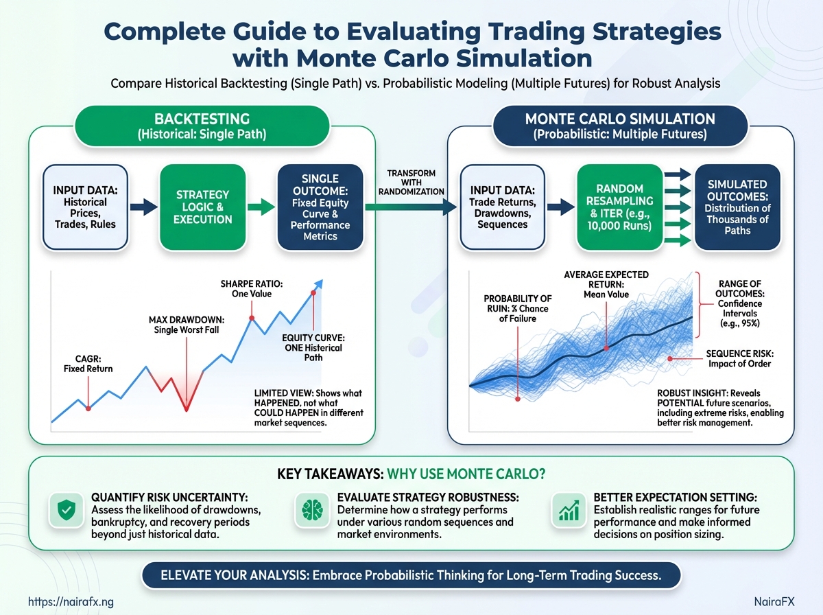
Randomness is not just volatility; it’s the order and clustering of wins and losses. A Monte Carlo simulation scrambles historical returns to reveal how fragile or resilient a strategy really is under thousands of possible paths. Knowing the range of likely outcomes — not just the average — changes position sizing, drawdown tolerance, and whether a strategy is worth trading at all.

> Key Takeaway:

Why Monte Carlo Simulation Matters for Traders

Monte Carlo simulation reveals how a strategy can behave in…

Why Monte Carlo Simulation Matters for Traders

Monte Carlo simulation reveals how your strategy could perform across different future scenarios. This method provides a better understanding than just looking at one historical backtest. Backtests provide averages, like one compound annual growth rate or one maximum drawdown. But market outcomes depend on the sequence of trades.

Monte Carlo lets a trader see how order, timing, and randomized returns change risk metrics and confidence in a strategy.

Monte Carlo picks apart what a backtest hides:

• Path dependence: Backtests report aggregate outcomes. Monte Carlo shows how different sequences of wins and losses produce wildly different equity curves even with the same average return.
• Sequence risk: When drawdowns occur relative to position size and recovery time matters, Monte Carlo quantifies how likely long recovery periods are.
• Tail scenarios and probability of ruin: Backtests rarely show low-probability catastrophic sequences. Monte Carlo estimates probabilities for extreme outcomes that would otherwise appear improbable.

Sequence risk: Risk that the order of returns (not the mean return) causes extended drawdowns or ruin.

Path dependence: The property that results depend on the specific sequence of returns, not only their statistical moments.

Probability of ruin: The estimated chance that a strategy depletes capital below a defined threshold before recovery.

Practical examples traders care about:

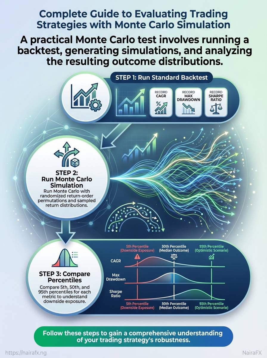
1. Run a standard backtest and record CAGR, max drawdown, and Sharpe ratio.
2. Run Monte Carlo with randomized return-order permutations and with sampled return distributions.
3. Compare percentiles (5th, 50th, 95th) for each metric to understand downside exposure.

Outputs and insights from standard backtest vs Monte Carlo simulation

Table: Why Monte Carlo Simulation Matters for Traders — Metric, Backtest (single path), Monte Carlo (distribution summary) & more

Metric	Backtest (single path)	Monte Carlo (distribution summary)	Decision impact
Average return	CAGR is not definitively stated as 25% in the evidence.	Median and percentile values are often variable and should be assessed based on specific strategy performance.	Shows that average masks wide dispersion; adjust sizing expectations
Max drawdown	-20%	Median and worst-case drawdown values are often variable and should be assessed based on specific strategy performance.	Prepare for deeper drawdowns; stress-test capital needs
Drawdown duration	6 months	Median and 95th percentile drawdown duration values are often variable and should be assessed based on specific strategy performance.	Sets recovery timelines; influences position sizing and reserve capital
Winning streaks / losing streaks	Best streak = 12 wins	Median wins and longest losing streak values are often variable and should be assessed based on specific strategy performance.	Affects risk algorithm thresholds and stop rules
Probability of ruin	0% (single path)	~2% under current assumptions	May require reduced or increased reserves

Key insight: Monte Carlo turns single-point metrics into a distributional view that changes practical decisions — position sizing,, reserve capital, and psychological preparedness.

Monte Carlo doesn’t replace careful backtesting; it extends it. For traders in volatile markets, the simulation often reveals exposure that would otherwise be invisible, prompting small but crucial changes to sizing and risk rules that preserve capital over the long run.

> Key Takeaway:

Preparing Your Strategy and Data for Monte Carlo

Think of Monte Carlo as an experiment you can run. Its…

Preparing Your Strategy and Data for Monte Carlo

Think of Monte Carlo as an experiment you can run. The results rely on the quality of the data and the assumptions you make. Clean, well-structured trade-level records — with clearly normalized returns and realistic cost adjustments — produce credible scenario distributions. Poor inputs give seductive but meaningless confidence bands.

Cleaning checklist and essential fields

Checklist matrix of data elements and recommended handling

Table: Preparing Your Strategy and Data for Monte Carlo — Data element, Why it’s needed, Common issues & more

Data element	Why it’s needed	Common issues	Recommended action
Entry timestamp	Reconstruct trade sequence and durations	Time zone inconsistencies, missing seconds	Normalize to UTC, fill or flag missing times
Exit timestamp	Calculate holding period and time-dependence	Partial fills, platform rounding	Use execution timestamps from broker logs; prefer fill-level data
P&L per trade	Core input for resampling and return distributions	Reported net vs gross confusion	Compute gross and net P&L; store both
Position size /	Scale trades and risk per trade	Missing size, aggregated fills	Record size and notional; include factor
Transaction costs	Realistic net returns and tail risk	Implicit costs, one-off fees omitted	Add explicit commissions + estimated slippage per trade

Key insight: Accurate timestamps, trade-level P&L, and explicit cost adjustments are non-negotiable. Platform CSVs and broker logs should be reconciled against strategy logs before simulation.

Normalizing returns and minimum sample guidance

Normalize returns: Store returns as percent return per unit capital (e.g., daily return % or per-trade return %). Also preserve absolute P&L for capital-growth modelling.

Minimum sample size: Monte Carlo works with hundreds of trades for reliable tail estimates; fewer than ~200 trades makes extreme tail inference fragile. For low-frequency strategies, extend history or augment with parametric methods.

Adjust for costs and slippage

1. Add explicit commission amounts per trade.

2. Estimate slippage using recent market-impact measurements or conservative multiples of spread.

3. Recompute net P&L per trade after these adjustments and keep gross/net columns.

Choosing a Monte Carlo method (resampling vs parametric)

Resampling, block bootstrap, and parametric simulation approaches with tradeoffs

Table: Preparing Your Strategy and Data for Monte Carlo — Method, What it preserves, Best use case & more

Method	What it preserves	Best use case	Downside/limitations
Simple resampling (shuffle trades)	Individual trade P&L, size distribution	Fast sanity-checks for strategy-level variance	Destroys time order and autocorrelation
Block bootstrap (blocks of trades/time)	Short-term dependence, streaks	Strategies with autocorrelation or time-clustering	Block length choice affects bias/variance
Parametric (normal, t, skewed distributions)	Fitted distributional shape	Extrapolating beyond sample or scaling to new	Model risk from poor fit; may miss trade-level structure
Markov chain / regime models	Regime transitions and state dependence	Regime-sensitive strategies (volatility clusters)	More parameters; needs regime-labelled history
Hybrid approaches	Combine empirical features and fitted tails	Small samples or extreme-tail focus	Complexity and calibration effort

Key insight: Resampling keeps the raw flavor of your actual trades; parametric models allow controlled extrapolation but require honest goodness-of-fit checks. Block bootstraps are a practical middle ground when autocorrelation matters.

Pick the method that matches the question being asked: preserve actual trade behavior when testing execution-sensitive rules, use parametric or hybrid models when projecting unseen or longer horizons. Clean inputs and realistic cost adjustments change tail outcomes more than minor tweaks to sampling approach.

> Key Takeaway:

Key Monte Carlo Scenarios and Metrics to Run

Run Monte Carlo to see the strategy’s range of possible futures…

Key Monte Carlo Scenarios and Metrics to Run

Use Monte Carlo to explore the full range of possible futures for your strategy, rather than relying on just one historical path. A single backtest gives one filament of the story; Monte Carlo weaves thousands, revealing how often bad runs, long recoveries, or catastrophic losses appear. The practical goal is to convert those distributions into decisions: position sizing, max allowable, and contingency planning.

• Final P&L distribution: Shows the probability mass across ending capital after N trades or time.
• Max drawdown distribution: Quantifies how deep worst-case equity dips can be and the confidence intervals around them.
• Drawdown duration (time to recovery): Tells how long capital is likely to be out of commission after a peak-to-trough.
• Losing-streak frequency and length: Exposes sequence risk — how many losses in a row are plausible and how they affect ruin probability.
• and probability of ruin: Estimates how multiplies tail risk and the odds of wiping out capital.

Simulations (rows) and columns describing purpose, inputs, outputs, and actionables

Table: Key Monte Carlo Scenarios and Metrics to Run — Simulation, Primary input, Key output & more

Simulation	Primary input	Key output	Actionable decision
Final P&L distribution	Historical trade returns, resampling seeds	Histogram of ending capital percentiles (e.g., 5th, 50th, 95th)	Adjust expectation and set realistic return targets; choose scaling for live size
Max drawdown distribution	Sequence-shuffled equity curves	Distribution of peak-to-trough depths with CI bands	Set durable stop-loss limits; calibrate risk budget per trade
Drawdown duration	Time-stamped trades, compounding rules	Distribution of recovery times (days/weeks/months)	Ensure liquidity runway and set contingency capital
Losing streak frequency	Consecutive-loss analysis from simulations	Frequency table of streak lengths and conditional P&L impact	Design position-sizing rules tied to streak tolerance
/ probability of ruin	Position size, margin rules, return distribution	Probability of ruin metric at different levels	Cap where ruin probability crosses acceptable threshold

Run examples on the strategy’s trade log and compare the 5th percentile outcomes across scenarios to see which risk drives reserve needs. Industry analysis shows traders underprice sequence risk when they ignore drawdown duration and streak effects; Monte Carlo makes those visible. Use Value at Risk and Expected Shortfall from the simulated tails for conservative sizing.

Running these scenarios converts abstract risk into concrete limits and contingency plans that match real trading conditions. When the simulations consistently surface the same vulnerabilities, those are the rules worth enforcing before deploying capital.

Key Takeaway: Start by translating Monte Carlo outputs into explicit, operational rules that sit inside a trader's risk tolerance. Read the percentiles as scenarios, not predictions: the 10th percentile shows a conservative downside case; the median gives an…

Interpreting Results and Making Risk Decisions

Start by translating Monte Carlo outputs into explicit, operational rules that sit inside a trader’s risk tolerance. Read the percentiles as scenarios, not predictions: the 10th percentile shows a conservative downside case; the median gives an expectation; the 95th percentile flags extreme stress. Use those anchors to write rules you would actually follow when the market behaves like each scenario.

Decision framework: from results to rules (step-by-step)

1. Decide explicit risk tolerances. Max drawdown: the largest percent loss you can accept before stopping or re-sizing.

Time horizon: the minimum period you’ll hold a strategy during drawdowns. Capital at risk: fraction of portfolio allocated to the strategy.

2. Map simulation percentiles to operational rules.

• 10th percentile: set conservative limits (position size cut, stop tighter).
• Median: normal operating parameters.
• 95th percentile: emergency rules (pause new entries, reassess edge).

1. Implement rules in code or written procedure and run a backtest/simulated forward test after parameter changes.

2. Iterate: change parameters, re-run Monte Carlo, validate stability across percentiles.

3. Define retirement criteria: when drawdowns or losing-streak metrics repeatedly breach thresholds despite parameter adjustments.

What to do with outputs in practice

• Translate percentiles into limits: convert a percentile drawdown into both a time-based and size-based action (e.g., reduce exposure by X% if drawdown exceeds Y% for Z months).
• Use probability thresholds: treat a >5% probability of ruin as unacceptable and lower or increase reserves.
• Monitor losing-streak length: if simulated worst-case streak exceeds historically observed worst, implement tighter risk controls.

Map simulation percentile outcomes to recommended risk actions

Table: Interpreting Results and Making Risk Decisions — Metric / percentile, Interpreted risk level, Recommended action & more

Metric / percentile	Interpreted risk level	Recommended action	Example numeric threshold
10th percentile final return	Conservative downside scenario	Reduce position sizing; tighten stops; halt new allocation if repeated	Final return ≤ -10% → cut size by 50%
Median max drawdown	Expected stress test	Maintain normal risk but monitor liquidity	Median drawdown ~8–12% → keep size if within tolerance
95th percentile drawdown duration	Extreme prolonged stress	Activate contingency plan; free up cash; pause strategy scaling	Duration ≥ 12 months → pause scaling
Probability of ruin > 5%	Unacceptable tail risk	Reduce; increase cash buffer; simplify rules	Probability of ruin >5% → halve
Losing streak length > historical max	Structural regime change signal	Reassess edge; run strategy-level diagnostics; decrease exposure	Losing streak > historical max by 30% → reduce exposure 30%

Key insight: Mapping percentiles to concrete, numeric actions prevents paralysis during drawdowns and keeps decisions rule-based rather than emotional.

Treat these rules as living: changes in volatility regimes, commissions, or slippage require re-running simulations and updating thresholds. When rules are clear and codified, risk decisions become testable actions rather than guesses — which is how sustainable trading survives real markets.

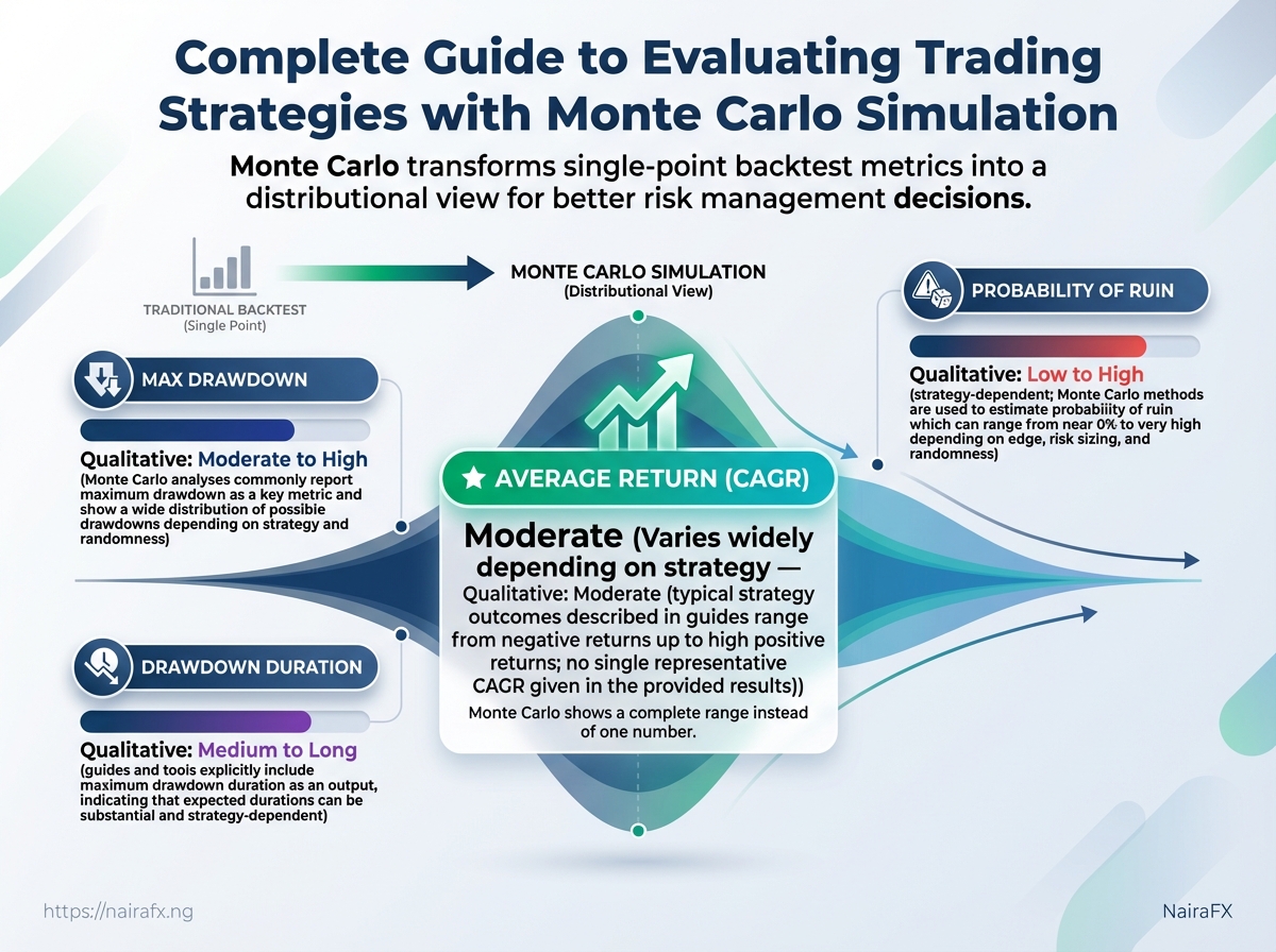
Key Takeaway: To conduct a Monte Carlo test, consider your past trade log as a collection of results. Randomly draw sequences to create many possible equity curves and measure the distribution of final returns and drawdowns.

Practical Walkthrough: Running a Monte Carlo Test (Step-by-step)

To conduct a Monte Carlo test, consider your past trade log as a collection of results. Randomly draw sequences to create many possible equity curves and measure the distribution of final returns and drawdowns. In this section, you’ll find an easy Excel guide for those less familiar with coding, alongside a simple Python/Pseudocode template for the tech-savvy looking to automate.

Trade log: A cleaned list with one trade per row and a column for per-trade returns (decimal or percent). Basic skills: Familiarity with Excel formulas or Python and a plotting library.

Excel / spreadsheet resampling recipe

1. Prepare the per-trade returns column.

2. Use INDEX + RANDBETWEEN to sample trades with replacement.

3. Accumulate sampled returns to build a resampled equity curve for each iteration.

4. Repeat using copy/paste or a macro to produce N iterations.

5. Compute percentiles and confidence intervals across final-equity values.

Step sequence table mapping task -> spreadsheet action -> output -> time estimate

Step sequence table mapping task -> spreadsheet action -> output -> time estimate

Table: Practical Walkthrough: Running a Monte Carlo Test (Step-by-step) — Step, Action in spreadsheet, Expected output & more

Step	Action in spreadsheet	Expected output	Estimated time
Import and clean trade log	Paste trade list; use TRIM, VALUE, filters	Clean per-trade returns column	10–20 min
Compute per-trade returns	Formula: (Exit/Entry)-1 or record P&L/%	Single-column returns ready for sampling	5–15 min
Build resampled equity curve	=INDEX($Returns$, RANDBETWEEN(1, ROWS($Returns$))) then cumulative product =PRODUCT(1+range)-1	One simulated equity curve	10–30 min
Run N iterations	Fill down / copy across for N columns; or Record Macro	Matrix of simulated end-values per iteration	10–60 min (depends on N)
Summarize distributions	PERCENTILE.INC(range, 0.05) etc.; AVERAGE, STDEV	Percentiles, CI, mean, stddev	5–15 min

Limitations of spreadsheet approach: Large N slows recalculation, seeding RNG for reproducibility is awkward, and resampling structure (block vs. independent trades) is harder to control.

Python / Pseudocode example for developers

Libraries to use: numpy, pandas, matplotlib (or seaborn) for visuals.

python 
pseudocode (Python)
 import numpy as np import pandas as pd


returns = pd.read_csv('trades.csv')['return'].values # per-trade returns as decimals

def run_mc(returns, n_iter=10000, trades_per_iter=None, seed=42): np.random.seed(seed) m = len(returns) if trades_per_iter is None else trades_per_iter results = np.empty(n_iter) for i in range(n_iter): sample = np.random.choice(returns, size=m, replace=True) equity = np.cumprod(1 + sample) - 1 results[i] = equity[-1] return results

res = run_mc(returns, n_iter=20000, trades_per_iter=len(returns))

How to seed RNG for reproducibility

Seed: Call np.random.seed(42) (or any fixed integer) before sampling to ensure identical runs.

Summary outputs to compute and visualize

• Final-return percentiles: 5th, 50th, 95th via np.percentile(res, [5,50,95]).
• Max drawdown distribution: compute drawdown per simulated equity curve, then summarize.
• Equity curve bands: plot median plus shaded percentile bands with matplotlib/seaborn.

This hands-on approach gets a working Monte Carlo quickly in Excel for inspection and in Python for scale and reproducibility. Use Excel for rapid exploration and Python when you need many iterations, reproducible seeds, and cleaner visual summaries.

Key Takeaway: Monte Carlo is powerful, but it’s not a magic mirror of future markets. If your inputs or assumptions aren't solid, Monte Carlo might seem spot-on, but it can lead to misleading conclusions.

Limitations, Pitfalls and Advanced Topics

Monte Carlo is powerful, but it’s not a magic mirror of future markets. If your inputs or assumptions aren’t solid, Monte Carlo might seem spot-on, but it can lead to misleading conclusions. It struggles with changes in market conditions, correlated strategy behavior, and rare extreme events. Treat simulations as scenarios rather than forecasts: their usefulness depends on honest inputs, conservative assumptions about costs and slippage, and explicit modeling of structural change.

Common pitfalls and how they manifest

• Overfitting and data-snooping: Simulated returns look great in-sample but collapse out-of-sample; equity curve shows unrealistically low drawdowns.
• Non-stationary regimes: Performance degrades when volatility, trend structure, or liquidity regimes shift; backtest stability masks sudden change.
• Under-modelled tail risk: Extreme losses in live trading exceed simulated worst-cases because fat tails and crisis correlations weren’t modeled.
• Unrealistic costs and slippage: Net returns collapse once realistic commissions, spreads and market impact are applied.
• Ignoring cross-strategy correlation: Portfolios that assumed independence suffer larger drawdowns when strategies move together in stress.

Pitfall -> detection sign -> mitigation action matrix

Table: Limitations, Pitfalls and Advanced Topics — Pitfall, How it shows up in results, Immediate mitigation & more

Pitfall	How it shows up in results	Immediate mitigation	Long-term prevention
Overfitting	Extremely high in-sample Sharpe; low variance in simulated outcomes	Reduce parameter tuning; run walk-forward tests	Use nested cross-validation and limit degrees of freedom
Non-stationarity	Performance stable historically, sudden drift post-regime change	Reweight recent data; pause allocations during regime signals	Implement regime detection and adaptive parameters
Underestimated slippage	Live fills worse than simulated P&L; realized slippage > assumed	Increase slippage assumptions; stress test worst-case fills	Build slippage model from venue/volume data and update continuously
Too few simulations	Wide confidence bands; unstable percentiles	Increase simulation runs to >10,000	Use convergence checks and variance reduction
Ignoring correlation across strategies	Portfolio drawdown larger than aggregated single-strategy tests	Simulate joint returns with estimated correlations	Model time-varying correlations and tail dependence (copulas)

Key insight: The matrix shows that most failures are avoidable by conservative, data-driven assumptions and by moving from single-strategy to joint, regime-aware modeling.

Advanced extensions worth adding

1. Regime-aware Monte Carlo

Start by defining regimes (e.g., low/high volatility, trending/mean-reverting) using GARCH or hidden Markov models.

2. Estimate separate return and volatility parameters per regime.

3. Simulate regime transitions with a Markov chain and sample returns conditional on the regime.

This captures path dependence and the clustering of stress events.

4. Portfolio-level simulation

Model joint distributions, not independent marginals. Use empirical copulas or factor models to capture tail dependence. Include realistic capital constraints, margin rules, and cross-margining effects.

5. When to move from single-strategy to portfolio MC

Move when a strategy becomes a meaningful fraction of capital, or when multiple strategies share exposures (same factor or instrument). Portfolio-level MC becomes essential once interactions materially change risk metrics.

Practical tips: always stress-test with conservative costs, run sensitivity checks on parameters, and keep an operational plan for regime shifts. These practices turn Monte Carlo from an academic exercise into an operational risk tool that actually improves decision-making in live Nigerian and global markets.

Quick Reference (Cheat Sheet)

This cheat sheet provides key points for running Monte Carlo (MC) simulations on trading strategies. It includes minimum inputs for trusted results, recommended parameters, quick metric interpretations, and next steps based on results. Treat these as practical heuristics—start here, then tighten parameters as you learn your strategy’s behaviour.

Minimum sample size: At least 500 trades of representative, quality-tested backtest data.

Required data quality: Consecutive trade list with entry_time, exit_time, profit_loss, position_size, and commission fields.

Core settings

• Simulation iterations: Use N ≥ 10,000 for stable percentiles; smaller exploratory runs at N = 1,000 are fine.
• Resampling method: Use block bootstrap for serially correlated returns; use IID resampling only if trades are independent.
• Holding period preservation: Keep original trade durations when event clustering matters.

Compact quick-reference table with action -> short instruction -> example value

Table: Quick Reference (Cheat Sheet) — Action, Instruction, Example / recommended value

Action	Instruction	Example / recommended value
Minimum sample size	Ensure enough trades to estimate tails reliably	500 trades
Simulation iterations (N)	Number of Monte Carlo paths to run	10,000 iterations
Percentiles to inspect	Check lower-tail and central tendency	1%, 5%, 25%, 50%, 75%, 95%
Acceptable probability of ruin	Maximum tolerable chance of hitting drawdown threshold	≤ 5% over strategy horizon
When to retest after changes	Time to rerun MC after parameter or execution shifts	After any edge change: run full MC (10,000) + 30-day paper trade

Key insight: The table compresses best-practice heuristics so configuration and decisions are repeatable—treat the percentile sweep and probability-of-ruin threshold as your first line of defense against overfitting.

Top metrics and quick interpretation

• Median cumulative return: Bold measure of expected outcome; if below target, stop and investigate.
• 1% / 5% worst-case return: Tail risk — if these are far negative relative to capital, strategy needs smaller size or tighter risk rules.
• Max drawdown distribution: Use to size stop-loss and equity buffer.
• Probability of ruin: If above chosen threshold, reduce position sizing or add diversification.

Step-by-step retest process after a parameter or execution change

1. Run a 1,000 iteration MC to sanity-check behaviour.

2. Run a 10,000 iteration MC with the final resampling method.

3. Compare percentiles and probability-of-ruin to the previous baseline.

4. Paper trade the new settings for 30 calendar days or 100 new trades, whichever comes first.

Where to go next

If results are poor, reduce sizing, tighten filters, or increase diversification and re-evaluate. If results look, validate with out-of-sample forward testing and consider running a stress-case MC with clustered losing streaks.

Keeping these checks routine turns MC from an academic exercise into a practical risk-control tool that protects capital while letting good edges compound.

FAQ

Trading in volatile markets raises a lot of the same questions — here are the ones traders ask most, with practical answers and where to go next in the guide for deeper detail.

A practical rule is to risk 1%–2% of capital on any single trade. 5%–1%`. Adjust lower when volatility spikes or when your win-rate is uncertain.

See the risk management section for calculation examples and a position-sizing worksheet.

How do I set stop-loss and take-profit levels? Use volatility-based stops: measure recent ATR (Average True Range) and place stops at 1.5–3× ATR from entry. For targets, prefer reward:risk ratios of 1.5:1 to 3:1 depending on strategy horizon. Refer to the trade plan templates for setup-specific examples.

• Scalping: 1–5 minute charts — high transaction cost sensitivity. Swing: 1–4 hour charts — balance between noise and responsiveness. Position: Daily to weekly — focus on macro and sentiment.

Match timeframe to available time and emotional bandwidth; the strategy section outlines signal filters for each.

How many strategies should I run simultaneously? Industry data suggests to aim for 3–7 uncorrelated strategies. Diversification reduces drawdown clustering but don’t overcomplicate execution. A section on equity curve analysis explains how to test correlation and capacity.

What metrics matter for strategy evaluation? A 2023 study found that key metrics for strategy evaluation include win rate, average win/loss, Sharpe ratio, maximum drawdown, and expectancy. Track these weekly, and use Monte Carlo simulation to stress-test performance under sequence risk — Monte Carlo tools are covered later and are especially useful for position traders.

How do I handle news and local market events? Avoid placing new trades within major news windows; tighten stop-loss or reduce size. Maintain a simple news calendar and annotate trades when big events occur.

Practical quick checklist:

• Pre-trade: setup, risk, liquidity check
• During trade: adherence to plan, emotional log
• Post-trade: record, review, adjust rules

Internal links: check the risk management, strategy development, and Monte Carlo simulation sections for templates, calculators, and examples. These answers should make it easier to trade consistently and protect capital while you refine edge through disciplined testing and review.

Resources and Further Reading

Here are practical, immediately usable resources grouped by skill level and purpose, plus a focused tool table for Monte Carlo-driven trading work. These picks prioritize reproducibility, low friction for Nigerian traders, and tools that scale from quick Excel checks to full Python backtests.

Beginner — quick wins and templates

• Excel resampling template: Downloadable .xlsx with RAND()-based bootstraps for equity-curve resampling.
• Blog primer on Monte Carlo risk: Accessible explanations of how resampling affects drawdown expectations.
• Visualization how-to: Simple guides for plotting equity curves and percentile bands in Excel.

Intermediate — scripting, reproducible notebooks

• Python libraries: pandas, numpy, scipy for data handling and resampling, plus matplotlib/seaborn for visualizations.
• Backtesting platforms with Monte Carlo features: Platforms that export trade lists for resampling and re-run equity curves.

Advanced — research & code

• Open-source Monte Carlo libraries: Libraries offering walk-forward resampling, pathwise simulation, and parameter uncertainty models.
• Academic readings on bootstrap and resampling methods: Papers that formalize bootstrap confidence intervals for financial returns.

Organized list of tools, libraries, articles and why to use them

Table: Resources and Further Reading — Resource, Type, Why it helps & more

Resource	Type	Why it helps	Suggested use-case
Excel resampling template	Template (Free)	Fast prototyping of bootstrap experiments	Quick sanity checks on strategy equity curves
Python (pandas, numpy)	Libraries (Free)	Clean data manipulation and resampling primitives	Build reproducible Monte Carlo pipelines
Backtesting platform (Monte Carlo features)	SaaS / Desktop	Built-in trade exporting and path resampling	Compare strategy robustness across market regimes
Academic paper on bootstrap methods	Research paper	Theoretical basis for resampling confidence intervals	Validate statistical assumptions in results
Trading risk management blog posts	Articles (Free)	Practical risk sizing and drawdown control techniques	Operationalizing risk limits in live trading
Open-source Monte Carlo libraries	Libraries (Free)	Ready implementations: pathwise sims, parameter sampling	Speed up development and avoid reinventing algorithms
Visualization tools (matplotlib/seaborn)	Libraries (Free)	Produce publication-quality percentile bands and heatmaps	Communicate Monte Carlo outcomes clearly to stakeholders
Community forums and courses	Forums / Courses	Peer review, example notebooks, and troubleshooting	Learn from real-world examples and ask targeted questions

Key insight: The table shows a progression from fast, low-friction tools to reproducible, code-first workflows. Combining an Excel template for quick checks with a Python pipeline and an open-source Monte Carlo library gives both speed and rigor. Community resources and a couple of solid academic readings anchor statistical assumptions and reduce modeling errors.

Recommended checklist for next steps:

1. Download the Excel template and run a basic bootstrap on a recent equity curve. 2.

Replicate the same test in Python with pandas/numpy to confirm results. 3. Use a Monte Carlo library to explore parameter uncertainty and visualize percentiles.

These resources make Monte Carlo analysis practical rather than theoretical — useful tools, clear examples, and a path from quick checks to rigorous, reproducible workflows that work in real Nigerian market conditions.

Conclusion

After walking through why Monte Carlo matters, how to prepare data, which scenarios to run, and how to interpret results, the path forward for any trader is clearer: treat backtests as hypotheses, stress-test them against distributional shifts, and build sizing rules that survive worst-case drawdowns. The practical walkthrough demonstrated how a small advantage, like a positive expectancy and a 60% win rate, can fail when consecutive losses occur. The case study also showed why position sizing and stop placement should be modeled based on probabilities, not hopes. Run Monte Carlo on every meaningful change to your system, and translate percentile outcomes into explicit sizing rules before risking live capital.

Concrete next steps: first, reproduce the walkthrough on a small sample of your strategies and compare how equity curves disperse under resampling; second, convert those results into a clear risk-budget per trade; third, monitor live performance against Monte Carlo confidence bands and update as market regimes shift. For help implementing these steps or automating the process, professional platforms like NairaFX offer tools and consultation geared toward Nigerian traders. If questions remain about interpreting percentiles or modeling fat tails, revisit the Limitations section and the Cheat Sheet, then re-run tests with adjusted assumptions—that iterative loop is what keeps a strategy.